About Classification
Supervised Classification
Working with the Sample Editor
The Sample Editor window is the principal tool for inputting samples. For a selected class, it shows histograms of selected features of samples in the currently active map. The same values can be displayed for all image objects at a certain level or all levels in the image object hierarchy.
You can use the Sample Editor window to compare the attributes or histograms of image objects and samples of different classes. It is helpful to get an overview of the feature distribution of image objects or samples of specific classes. The features of an image object can be compared to the total distribution of this feature over one or all image object levels.
Use this tool to assign samples using a Nearest Neighbor classification or to compare an image object to already existing samples, in order to determine to which class an image object belongs. If you assign samples, features can also be compared to the samples of other classes. Only samples of the currently active map are displayed.
- Open the Sample Editor window using Classification > Samples > Sample Editor from the main menu
- By default, the Sample Editor window shows diagrams for only a selection of features. To select the features to be displayed in the Sample Editor, right-click in the Sample Editor window and select Select Features to Display
- In the Select Displayed Features dialog box, double-click a feature from the left-hand pane to select it. To remove a feature, click it in the right-hand pane
- To add the features used for the Standard Nearest Neighbor expression, select Display Standard Nearest Neighbor Features from the context menu.
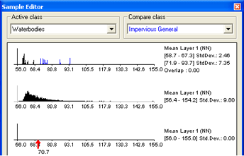
The Sample Editor window. The first graph shows the Active Class and Compare Class histograms. The second is a histogram for all image object levels. The third graph displays an arrow indicating the feature value of a selected image object
Comparing Features
To compare samples or layer histograms of two classes, select the classes or the levels you want to compare in the Active Class and Compare Class lists.
Values of the active class are displayed in black in the diagram, the values of the compared class in blue. The value range and standard deviation of the samples are displayed on the right-hand side.
Viewing the Value of an Image Object
When you select an image object, the feature value is highlighted with a red pointer. This enables you to compare different objects with regard to their feature values. The following functions help you to work with the Sample Editor:
- The feature range displayed for each feature is limited to the currently detected feature range. To display the whole feature range, select Display Entire Feature Range from the context menu
- To hide the display of the axis labels, deselect Display Axis Labels from the context menu
- To display the feature value of samples from inherited classes, select Display Samples from Inherited Classes
- To navigate to a sample image object in the map view, click on the red arrow in the Sample Editor.
In addition, the Sample Editor window allows you to generate membership functions. The following options are available:
- To insert a membership function to a class description, select Display Membership Function > Compute from the context menu
- To display membership functions graphs in the histogram of a class, select Display Membership Functions from the context menu
- To insert a membership function or to edit an existing one for a feature, select the feature histogram and select Membership Function > Insert/Edit from the context menu
- To delete a membership function for a feature, select the feature histogram and select Membership Function > Delete from the context menu
- To edit the parameters of a membership function, select the feature histogram and select Membership Function > Parameters from the context menu.
Selecting Samples
A Nearest Neighbor classification needs training areas. Therefore, representative samples of image objects need to be collected.
- To assign sample objects, activate the input mode. Choose Classification > Samples > Select Samples from the main menu bar. The map view changes to the View Samples mode.
- To open the Sample Editor window, which helps to gather adequate sample image objects, do one of the following:
- Choose Classification > Samples > Sample Editor from the main menu.
- Choose View > Sample Editor from the main menu.
- To select a class from which you want to collect samples, do one of the following:
- Select the class in the Class Hierarchy window if available.
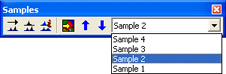
**Select the class from the Active Class drop-down list in the Sample Editor window.
This makes the selected class your active class so any samples you collect will be assigned to that class.
- To define an image object as a sample for a selected class, double-click the image object in the map view. To undo the declaration of an object as sample, double-click it again. You can select or deselect multiple objects by holding down the Shift key.
As long as the sample input mode is activated, the view will always change back to the Sample View when an image object is selected. Sample View displays sample image objects in the class color; this way the accidental input of samples can be avoided.
- To view the feature values of the sample image object, go to the Sample Editor window. This enables you to compare different image objects with regard to their feature values.
- Click another potential sample image object for the selected class. Analyze its membership value and its membership distance to the selected class and to all other classes within the feature space. Here you have the following options:
- The potential sample image object includes new information to describe the selected class: low membership value to selected class, low membership value to other classes.
- The potential sample image object is really a sample of another class: low membership value to selected class, high membership value to other classes.
- The potential sample image object is needed as sample to distinguish the selected class from other classes: high membership value to selected class, high membership value to other classes.
In the first iteration of selecting samples, start with only a few samples for each class, covering the typical range of the class in the feature space. Otherwise, its heterogeneous character will not be fully considered.
- Repeat the same for remaining classes of interest.
- Classify the scene.
- The results of the classification are now displayed in the map view. In the View Settings dialog box, the mode has changed from Samples to Classification.
- Note that some image objects may have been classified incorrectly or not at all. All image objects that are classified are displayed in the appropriate class color. If you hover the cursor over a classified image object, a tool -tip pops up indicating the class to which the image object belongs, its membership value, and whether or not it is a sample image object. Image objects that are unclassified appear transparent. If you hover over an unclassified object, a tool-tip indicates that no classification has been applied to this image object. This information is also available in the Classification tab of the Image Object Information window.
- The refinement of the classification result is an iterative process:
- First, assess the quality of your selected samples
- Then, remove samples that do not represent the selected class well and add samples that are a better match or have previously been misclassified
- Classify the scene again
- Repeat this step until you are satisfied with your classification result.
- When you have finished collecting samples, remember to turn off the Select Samples input mode. As long as the sample input mode is active, the viewing mode will automatically switch back to the sample viewing mode, whenever an image object is selected. This is to prevent you from accidentally adding samples without taking notice.
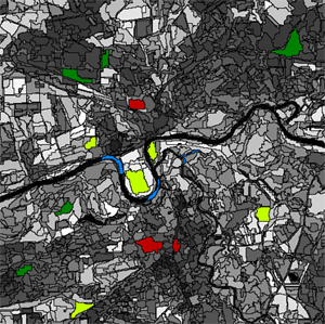
Map view with selected samples in View Samples mode. (Image data courtesy of Ministry of Environmental Affairs of Sachsen-Anhalt, Germany.)
Assessing the Quality of Samples
Once a class has at least one sample, the quality of a new sample can be assessed in the Sample Selection Information window. It can help you to decide if an image object contains new information for a class, or if it should belong to another class.
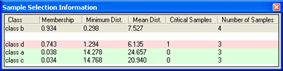
The Sample Selection Information window.
- To open the Sample Selection Information window choose Classification > Samples > Sample Selection Information or View > Sample Selection Information from the main menu
- Names of classes are displayed in the Class column. The Membership column shows the membership value of the Nearest Neighbor classifier for the selected image object
- The Minimum Dist. column displays the distance in feature space to the closest sample of the respective class
- The Mean Dist. column indicates the average distance to all samples of the corresponding class
- The Critical Samples column displays the number of samples within a critical distance to the selected class in the feature space
- The Number of Samples column indicates the number of samples selected for the corresponding class.
The following highlight colors are used for a better visual overview: - Gray: Used for the selected class.
- Red: Used if a selected sample is critically close to samples of other classes in the feature space.
- Green: Used for all other classes that are not in a critical relation to the selected class.
The critical sample membership value can be changed by right-clicking inside the window. Select Modify Critical Sample Membership Overlap from the context menu. The default value is 0.7, which means all membership values higher than 0.7 are critical.
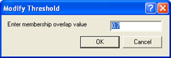
The Modify Threshold dialog box
To select which classes are shown, right-click inside the dialog box and choose Select Classes to Display.
Navigating Samples
To navigate to samples in the map view, select samples in the Sample Editor window to highlight them in the map view.
- Before navigating to samples you must select a class in the Select Sample Information dialog box.
- To activate Sample Navigation, do one of the following:
- Choose Classification > Samples > Sample Editor Options > Activate Sample Navigation from the main menu
- Right-click inside the Sample Editor and choose Activate Sample Navigation from the context menu.
- To navigate samples, click in a histogram displayed in the Sample Editor window. A selected sample is highlighted in the map view and in the Sample Editor window.
- If there are two or more samples so close together that it is not possible to select them separately, you can use one of the following:
- Select a Navigate to Sample button.
- Select from the sample selection drop-down list.
For sample navigation choose from a list of similar samples
Deleting Samples
- Deleting samples means to unmark sample image objects. They continue to exist as regular image objects.
- To delete a single sample, double-click or Shift-click it.
- To delete samples of specific classes, choose one of the following from the main menu:
- Classification > Class Hierarchy > Edit Classes > Delete Samples, which deletes all samples from the currently selected class.
- Classification > Samples > Delete Samples of Classes, which opens the Delete Samples of Selected Classes dialog box. Move the desired classes from the Available Classes to the Selected Classes list (or vice versa) and click OK
- To delete all samples you have assigned, select Classification > Samples > Delete All Samples.
Alternatively you can delete samples by using the Delete All Samples algorithm or the Delete Samples of Class algorithm.
Training and Test Area Masks
Existing samples can be stored in a file called a training and test area (TTA) mask, which allows you to transfer them to other scenes.
To allow mapping samples to image objects, you can define the degree of overlap that a sample image object must show to be considered within in the training area. The TTA mask also contains information about classes for the map. You can use these classes or add them to your existing class hierarchy.
Creating and Saving a TTA Mask
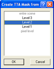
The Create TTA Mask from Samples dialog box
- From the main menu select Classification > Samples > Create TTA Mask from Samples
- In the dialog box, select the image object level that contains the samples that you want to use for the TTA mask. If your samples are all in one image object level, it is selected automatically and cannot be changed
- Click OK to save your changes. Your selection of sample image objects is now converted to a TTA mask
- To save the mask to a file, select Classification > Samples > Save TTA Mask. Enter a file name and select your preferred file format.
Loading and Applying a TTA Mask
To load samples from an existing Training and Test Area (TTA) mask:
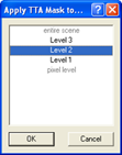
Apply TTA Mask to Level dialog box
- From the main menu select Classification > Samples > Load TTA Mask.
- In the Load TTA Mask dialog box, select the desired TTA Mask file and click Open.
- In the Load Conversion Table dialog box, open the corresponding conversion table file. The conversion table enables mapping of TTA mask classes to existing classes in the currently displayed map. You can edit the conversion table.
- Click Yes to create classes from the conversion table. If your map already contains classes, you can replace them with the classes from the conversion file or add them. If you choose to replace them, your existing class hierarchy will be deleted.
If you want to retain the class hierarchy, you can save it to a file.
- Click Yes to replace the class hierarchy by the classes stored in the conversion table.
- To convert the TTA Mask information into samples, select Classification > Samples > Create Samples from TTA Mask. The Apply TTA Mask to Level dialog box opens.
- Select which level you want to apply the TTA mask information to. If the project contains only one image object level, this level is preselected and cannot be changed.
- In the Create Samples dialog box, enter the Minimum Overlap for Sample Objects and click OK.
The default value is 0.75. Since a single training area of the TTA mask does not necessarily have to match an image object, the minimum overlap decides whether an image object that is not 100% within a training area in the TTA mask should be declared a sample.
The value 0.75 indicates that 75% of an image object has to be covered by the sample area for a certain class given by the TTA mask in order for a sample for this class to be generated.
The map view displays the original map with sample image objects selected where the test area of the TTA mask have been.
The Edit Conversion Table
You can check and edit the linkage between classes of the map and the classes of a Training and Test Area (TTA) mask.
You must edit the conversion table only if you chose to keep your existing class hierarchy and used different names for the classes. A TTA mask has to be loaded and the map must contain classes.
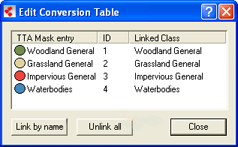
Edit Conversion Table dialog box
- To edit the conversion table, choose Classification > Samples > Edit Conversion Table from the main menu
- The Linked Class list displays how classes of the map are linked to classes of the TTA mask. To edit the linkage between the TTA mask classes and the classes of the current active map, right-click a TTA mask entry and select the appropriate class from the drop-down list
- Choose Link by name to link all identical class names automatically. Choose Unlink all to remove the class links.
Creating Samples Based on a Shapefile
You can use shapefiles to create sample image objects. A shapefile, also called an ESRI shapefile, is a standardized vector file format used to visualize geographic data. You can obtain shapefiles from other geo applications or by exporting them from eCognition maps. A shapefile consists of several individual files such as .shx, .shp and .dbf.
To provide an overview, using a shapefile for sample creation comprises the following steps:
- Opening a project and loading the shapefile as a thematic layer into a map
- Segmenting the map using the thematic layer
- Classifying image objects using the shapefile information.
Creating the Samples
Edit a process to use a shapefile
Add a shapefile to an existing project
- Open the project and select a map
- Select File > Modify Open Project from the main menu. The Modify Project dialog box opens
- Insert the shapefile as a new thematic layer. Confirm with OK.
Add a Parent Process
- Go to the Process Tree window
- Right-click the Process Tree window and select Append New
- Enter a process name. From the Algorithm list select Execute Child Processes, then select Execute in the Domain list.
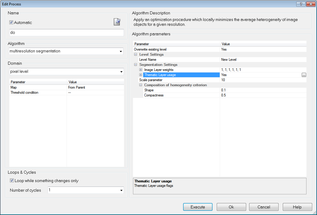
Add segmentation Child Process
- In the Process Tree window, right-click and select Insert Child from the context menu
- From the Algorithm drop-down list, select Multiresolution Segmentation. Under the segmentation settings, select Yes in the Thematic Layer entry.
The segmentation finds all objects of the shapefile and converts them to image objects in the thematic layer.
Classify objects using shapefile information
- For the classification, create a new class (for example ‘Sample’)
- In the Process Tree window, add another process.
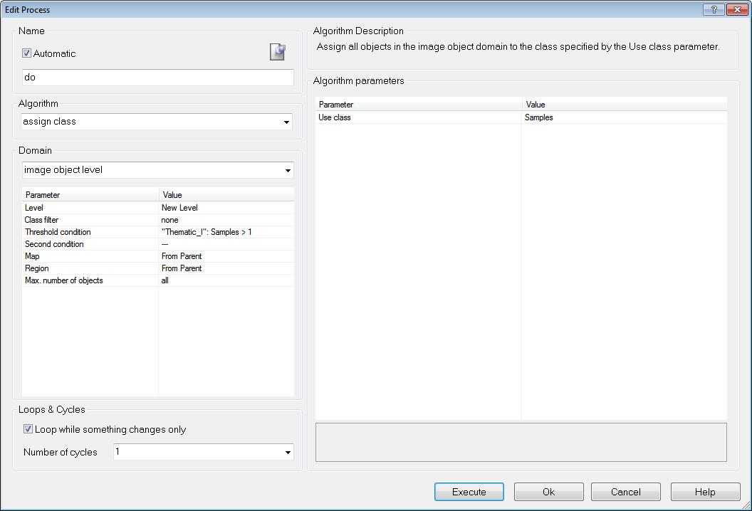
The child process identifies image objects using information from the thematic layer – use the threshold classifier and a feature created from the thematic layer attribute table, for example ‘Image Object ID’ or ‘Class’ from a shapefile ‘Thematic Layer 1’
- Select the following feature: Object Features > Thematic Attributes > Thematic Object Attribute > [Thematic Layer 1]
- Set the threshold to, for example, > 0 or = “Sample” according to the content of your thematic attributes
- For the parameter Use Class, select the new class for assignment.
Converting Objects to samples
- To mark the classified image objects as samples, add another child process
- Use the classified image objects to samples algorithm. From the Domain list, select New Level. No further conditions are required
- Execute the process.
Process to import samples from shapefile
Selecting Samples with the Sample Brush
The Sample Brush is an interactive tool that allows you to use your cursor like a brush, creating samples as you sweep it across the map view. Go to the Sample Editor toolbar (View > Toolbars > Sample Editor) and press the Select Sample button. Right-click on the image in map view and select Sample Brush.
Drag the cursor across the scene to select samples. By default, samples are not reselected if the image objects are already classified but existing samples are replaced if drag over them again. These settings can be changed in the Sample Brush group of the Options dialog box. To deselect samples, press Shift as you drag.
The Sample Brush will select up to one hundred image objects at a time, so you may need to increase magnification if you have a large number of image objects.
Setting the Nearest Neighbor Function Slope
The Nearest Neighbor Function Slope defines the distance an object may have from the nearest sample in the feature space while still being classified. Enter values between 0 and 1. Higher values result in a larger number of classified objects.
- To set the function slope, choose Classification > Nearest Neighbor > Set NN Function Slope from the main menu bar.
- Enter a value and click OK.
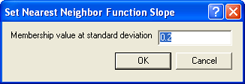
The Set Nearest Neighbor Function Slope dialog box
Using Class-Related Features in a Nearest Neighbor Feature Space
To prevent non-deterministic classification results when using class-related features in a nearest neighbor feature space, several constraints have to be mentioned:
- It is not possible to use the feature Similarity To with a class that is described by a nearest neighbor with class-related features.
- Classes cannot inherit from classes that use nearest neighbor-containing class-related features. Only classes at the bottom level of the inheritance class hierarchy can use class-related features in a nearest neighbor.
- It is impossible to use class-related features that refer to classes in the same group including the group class itself.
Classifier Algorithms
Overview
The classifier algorithm allows classifying based on different statistical classification algorithms:
- Bayes
- KNN (K Nearest Neighbor)
- SVM (Support Vector Machine)
- Decision Tree
- Random Trees
The Classifier algorithm can be applied either pixel- or object-based. For an example project containing these classifiers please refer here http://community.ecognition.com/home/CART%20-%20SVM%20Classifier%20Example.zip/view
Bayes
A Bayes classifier is a simple probabilistic classifier based on applying Bayes’ theorem (from Bayesian statistics) with strong independence assumptions. In simple terms, a Bayes classifier assumes that the presence (or absence) of a particular feature of a class is unrelated to the presence (or absence) of any other feature. For example, a fruit may be considered to be an apple if it is red, round, and about 4” in diameter. Even if these features depend on each other or upon the existence of the other features, a Bayes classifier considers all of these properties to independently contribute to the probability that this fruit is an apple. An advantage of the naive Bayes classifier is that it only requires a small amount of training data to estimate the parameters (means and variances of the variables) necessary for classification. Because independent variables are assumed, only the variances of the variables for each class need to be determined and not the entire covariance matrix.
KNN (K Nearest Neighbor)
The k-nearest neighbor algorithm (k-NN) is a method for classifying objects based on closest training examples in the feature space. k-NN is a type of instance-based learning, or lazy learning where the function is only approximated locally and all computation is deferred until classification. The k-nearest neighbor algorithm is amongst the simplest of all machine learning algorithms: an object is classified by a majority vote of its neighbors, with the object being assigned to the class most common amongst its k nearest neighbors (k is a positive integer, typically small). The 5-nearest-neighbor classification rule is to assign to a test sample the majority class label of its 5 nearest training samples. If k = 1, then the object is simply assigned to the class of its nearest neighbor.
This means k is the number of samples to be considered in the neighborhood of an unclassified object/pixel. The best choice of k depends on the data: larger values reduce the effect of noise in the classification, but the class boundaries are less distinct.
eCognition software has the Nearest Neighbor implemented as a classifier that can be applied using the algorithm classifier (KNN with k=1) or using the concept of classification based on the Nearest Neighbor Classification.
SVM (Support Vector Machine)
A support vector machine (SVM) is a concept in computer science for a set of related supervised learning methods that analyze data and recognize patterns, used for classification and regression analysis. The standard SVM takes a set of input data and predicts, for each given input, which of two possible classes the input is a member of. Given a set of training examples, each marked as belonging to one of two categories, an SVM training algorithm builds a model that assigns new examples into one category or the other. An SVM model is a representation of the examples as points in space, mapped so that the examples of the separate categories are pided by a clear gap that is as wide as possible. New examples are then mapped into that same space and predicted to belong to a category based on which side of the gap they fall on. Support Vector Machines are based on the concept of decision planes defining decision boundaries. A decision plane separates between a set of objects having different class memberships.
Important parameters for SVM
There are different kernels that can be used in Support Vector Machines models. Included in eCognition are linear and radial basis function (RBF). The RBF is the most popular choice of kernel types used in Support Vector Machines. Training of the SVM classifier involves the minimization of an error function with C as the capacity constant.
Decision Tree (CART resp. classification and regression tree)
Decision tree learning is a method commonly used in data mining where a series of decisions are made to segment the data into homogeneous subgroups. The model looks like a tree with branches - while the tree can be complex, involving a large number of splits and nodes. The goal is to create a model that predicts the value of a target variable based on several input variables. A tree can be “learned” by splitting the source set into subsets based on an attribute value test. This process is repeated on each derived subset in a recursive manner called recursive partitioning. The recursion is completed when the subset at a node all has the same value of the target variable, or when splitting no longer adds value to the predictions. The purpose of the analyses via tree-building algorithms is to determine a set of if-then logical (split) conditions.
Important Decision Tree parameters
The minimum number of samples that are needed per node are defined by the parameter Min sample count. Finding the right sized tree may require some experience. A tree with too few of splits misses out on improved predictive accuracy, while a tree with too many splits is unnecessarily complicated. Cross validation exists to combat this issue by setting eCognitions parameter Cross validation folds. For a cross-validation the classification tree is computed from the learning sample, and its predictive accuracy is tested by test samples. If the costs for the test sample exceed the costs for the learning sample this indicates poor cross-validation and that a different sized tree might cross-validate better.
Random Trees
The random trees classifier is more a framework that a specific model. It uses an input feature vector and classifies it with every tree in the forest. It results in a class label of the training sample in the terminal node where it ends up. This means the label is assigned that obtained the majority of "votes". Iterating this over all trees results in the random forest prediction. All trees are trained with the same features but on different training sets, which are generated from the original training set. This is done based on the bootstrap procedure: for each training set the same number of vectors as in the original set ( =N ) is selected. The vectors are chosen with replacement which means some vectors will appear more than once and some will be absent. At each node not all variables are used to find the best split but a randomly selected subset of them. For each node a new subset is construced, where its size is fixed for all the nodes and all the trees. It is a training parameter, set to  . None of the trees that are built are pruned.
In random trees the error is estimated internally during the training. When the training set for the current tree is drawn by sampling with replacement, some vectors are left out. This data is called out-of-bag data - in short "oob" data. The oob data size is about N/3. The classification error is estimated based on this oob-data.
Classification using the Template Matching Algorithm
As described in the Reference Book > Template Matching you can apply templates generated with eCognitions Template Matching Editor to your imagery.
Please refer to our template matching videos in the eCognition community http://www.ecognition.com/community covering a variety of application examples and workflows.
The typical workflow comprises two steps. Template generation using the template editor, and template application using the template matching algorithm.
To generate templates:
- Create a new project
- Open View > Windows > Template Editor
- Insert samples in the Select Samples tab
- Generate template(s) based on the first samples selected
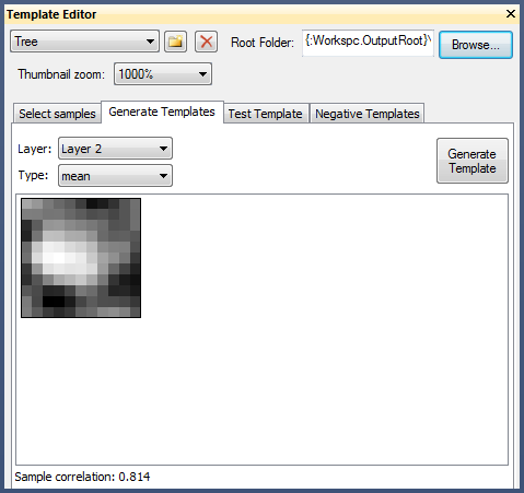
Exemplary Tree Template in the Template Editor
- Test the template on a subregion resulting in potential targets
- Review the targets and assign them manually as correct, false or not sure (note that targets classified as correct automatically become samples)
- Regenerate the template(s) on this improved sample basis
- Repeat these steps with varying test regions and thresholds, and improve your template(s) iteratively
- Save the project (saves also the samples)
To apply your templates:
- Create a new project/workspace with imagery to apply the templates to
- Insert the template matching algorithm in the Process Tree Window
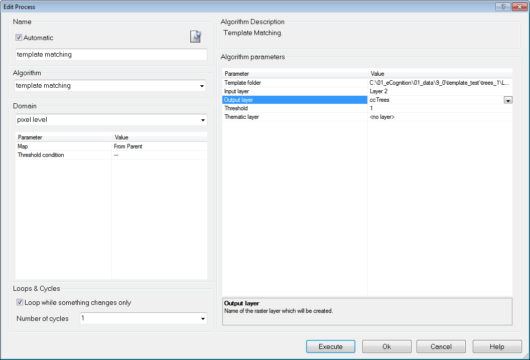
Template Matching Algorithm to generate Correlation Coefficient Image Layer
- To generate the a temporary layer with correlation coefficients (output layer) you need to provide
- the folder containing the template(s)
- the layer that should be correlated with this template
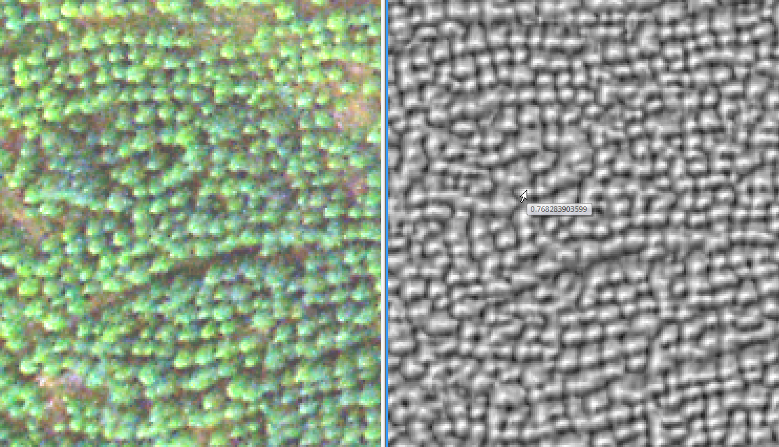
RGB Image Layer (left) and Correlation Coefficient Image Layer (right)
- To generate in addition a thematic layer with points for each target you need to provide a threshold for the correlation coefficient for a valid target
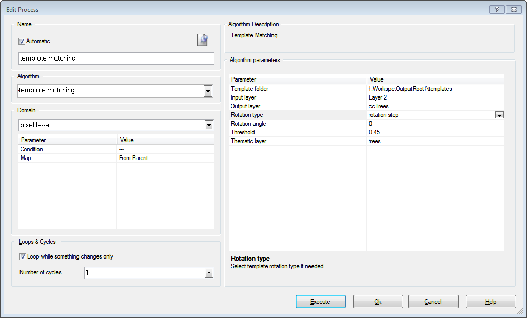
Template Matching Algorithm to generate Thematic Layer with Results
- Apply the template matching algorithm
- Segment your image based on the thematic layer and use the “assign class by thematic layer” algorithm to classify your objects
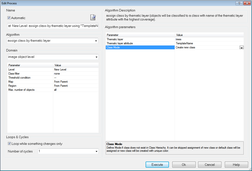
Assign Classification by Thematic Layer Algorithm
- Review your targets using the image object table (zoom in and make only a small region of the image visible, and any object you select in the table will be visible in the image view, typically centered).
